How to color alternate rows in Excel, a tutorial to make it easier to analyze the datasheet and make the graphics more enjoyable.
It has already happened to you several times to see rows or columns of alternating colors on Excel sheets and I am sure you have asked yourself: but how did they do it? Quiet, nothing easier.
In the latest versions of Excel it is possible to apply a preset format where the background of alternating rows or columns applies automatically as soon as you add rows and columns.

In this article I will explain how to color alternate rows in Excel improving their readability through three simple ways: the command Format as a table, conditional formatting, and using VBA to create lines of code to customize the table.
How to color alternate rows in Excel with Format as Table
Using this mode is very simple. Open Excel and select in the sheet you are working on the range of cells you want to format.
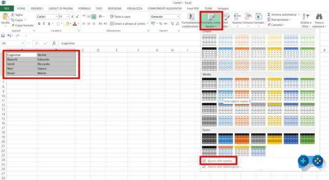
Then go to the menu Home> Format as a table. You will find a number of table styles with alternating rows to apply. Choose one and that's it. Remember to tick the box before confirming Tables with headers after choosing the style.
If you want to switch between alternating rows and alternating columns style, select the entire table and click Planning. Uncheck the box Righe age. evidence. and check the box Colonne age. evidence..

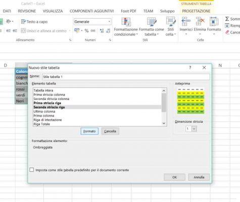
To customize the color of alternating rows in Excel go to Home> Format as Table> New Table Style. Here you can select First strip line and click on the button Size to choose the fill color and immediately after Second row strip and perform the same operation. Confirm by pressing the button Ok.
In case you need to add new rows to the table with alternating rows, you will have to copy the alternating color formats in the new rows using the command Format Painter. Select the last two lines, then press the icon at the top, in the Home, of Copy format and positioned on the last empty line and then right-click on Paste in the pop-up menu (or CTRL + V).
 How to view the formulas of an Excel sheet
How to color alternate rows in Excel with Conditional Formatting
Another way to have alternating colored rows in an Excel table is through a conditional formatting rule.
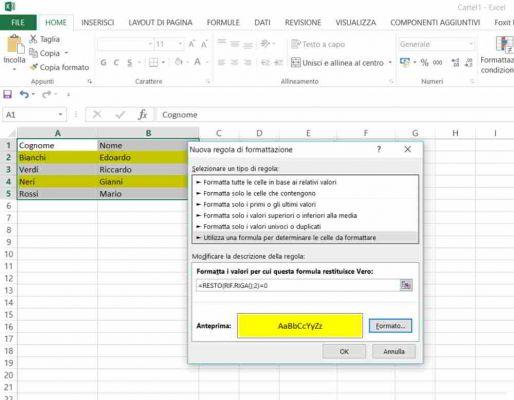
Select the range of cells you want to format (you can also select the whole sheet with the button Select all) and go up Home> Conditional Formatting> New Rule.
Then select the type of rule Use a formula to determine which cells to format, in the window Select a rule type. In the field Format the values for which this formula returns True, type = REST (ROW (); 2) = 0. Press the button Size and choose a fill color. Then press OK to view the result obtained.
To have alternating columns of color, the command is = REST (COLUMN REF (); 2) = 0.
With conditional formatting, adding new rows or columns will automatically insert the fill color.
To change the Conditional Formatting, you need to go to Home > Conditional formatting > Manage rules > Edit rule, if you want to remove conditional formatting instead, always go to Home > Conditional Formatting> Clear Rules and choose one of the two commands between Clear rules from selected cells or Delete rules from whole sheet.
 How to add photos in Excel lists
How to color alternate rows in Excel with Format with VBA
For experts of Macro VBA in Excel, here is a little function to play with and which you can modify as you like:
SubColoringAlternate Stripes ()
Range(“A2:B10”).Interior.ColorIndex = 2
For j= 2 To 10 Step 2
Range(“A” & j & “:B” & j).Interior.ColorIndex = 36
Next j
End Sub
 Free Excel Family Budget Templates